AVL & Splay & Amortized Analysis👀
约 1529 个字 7 行代码 预计阅读时间 5 分钟
AVL Trees👀
也可称为 Blanced Binary Search Trees (BBST) | AVL (Adelson-Velsky and Landis) Trees
Definitions
- An empty binary tree is height balanced. If \(T\) is a nonempty binary tree with \(T_L\) and \(T_R\) as its left and right subtrees, then \(T\) is height balanced if
- \(T_L\) and \(T_R\) are height balanced, and
- \(| h_L - h_R | \le 1\) where \(h_L\) and \(h_R\) are heights of \(T_L\) and \(T_R\)
- The balanced factor \(BF\) (node) = \(h_L - h_R\). In an AVL tree, \(BF\) (node) = -1, 0, or 1
Maximum Height👀
- Let \(n_h\) be the minimum number of nodes in a balanced binary tree with height \(h\)
- 结点数最小时:
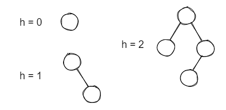
- In genernal ( \(n_h = n_{h-1} + n_{h-2} + 1\) ):
- Cause Fibonacci sequence: \(F_0 = 1, ~ F_1 = 1, ~ F_i = F_{i-1} + F_{i-2}\) for \(i > 1\)
- \(n_h = n_{h-1} + n_{h-2} + 1 ~~ \Rightarrow ~~ n_h = F_{h+2} - 1 (h \ge 0)\)
- \(F_i ~ \approx ~ \frac{1}{\sqrt{5}} ( \frac{1+\sqrt{5}}{2} )^i ~~ \Rightarrow ~~ n_h ~ \approx ~ \frac{1}{\sqrt{5}} ( \frac{1+\sqrt{5}}{2} )^{h+2} - 1 ~~ \Rightarrow ~~ h = O(log ~ n_h)\)
- \(n \ge n_h ~~ \Rightarrow ~~ h = O(log ~ n)\)
- 结点数最小时:
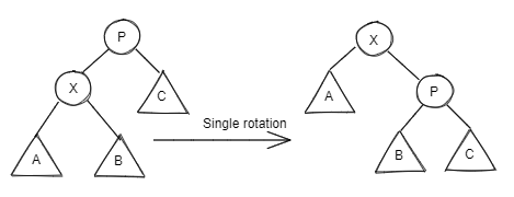
Rotation👀
RR👀
Single Rotation
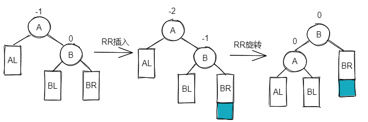
依次插入 Mar, May, Nov
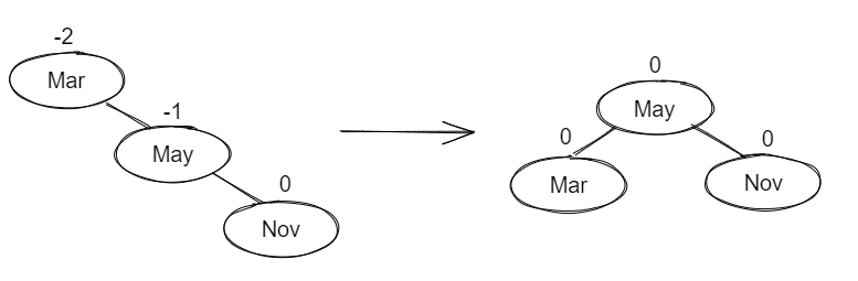
不平衡的 “发现者” 是 Mar, “麻烦结点” Nov 在发现者的右子树的右边,因而叫 “RR 插入”,需要 “RR 旋转” 即右单旋
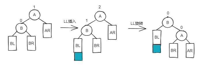
LL👀
Single Rotation
再依次插入 Aug, Apr
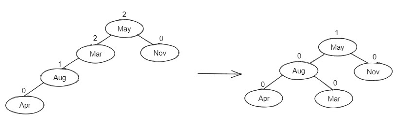
“发现者” 是 Mar, “麻烦结点” Apr 在发现者的左子树的左边,因而叫 “LL 插入”,需要 “LL 旋转” 即左单旋
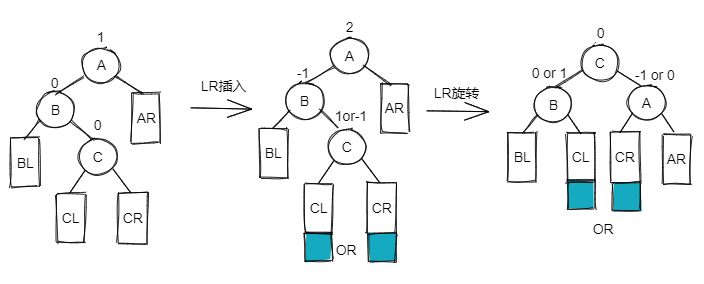
LR👀
Double Rotation
再插入 Jan
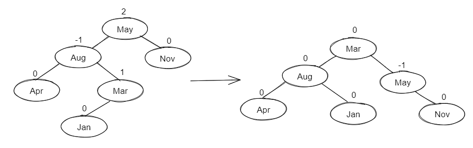
“发现者” 是 May, “麻烦结点” Jan 在发现者的左子树的右边,因而叫 “LR 插入”,需要 “LR 旋转”
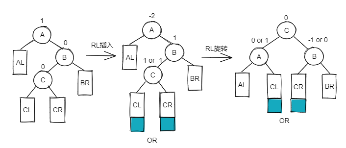
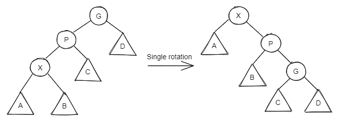
RL👀
Double Rotation
再插入 Dec, July, Feb
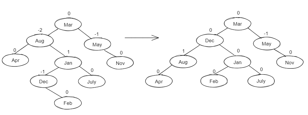
“发现者” 是 Aug, “麻烦结点” Feb 在发现者的右子树的左边,因而叫 “RL 插入”,需要 “RL 旋转”
Splay Trees & Amortized Analysis👀
Splay Trees | 伸展树👀
Splay Tree - Definition
A relatively simple date structure, known as splay tree, that guarantees that any m consecutive tree operations take at most \(O(Mlog~N)\) time.
It means that the amortized time is \(O(log~N)\)
Any simgle operation might take \(O(N)\) time
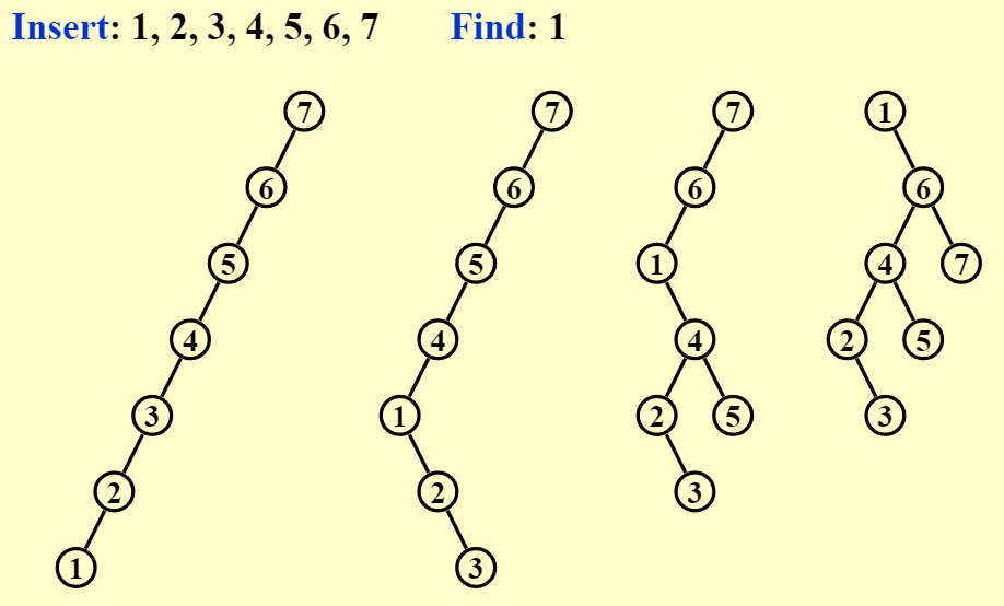
Find👀
- 伸展树的核心想法是: 一个节点被访问后,通过一系列 AVL Tree 的旋转方法将它转至根节点
- 尝试单旋:
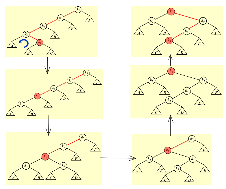
- 发现 K3 沉到了更底部
-
给出新的旋转方法:
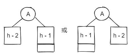
For any nonroot node X, denote its parent by P and grandparent by G:
- Case 1: P is the root ——> Rotate X and P
-
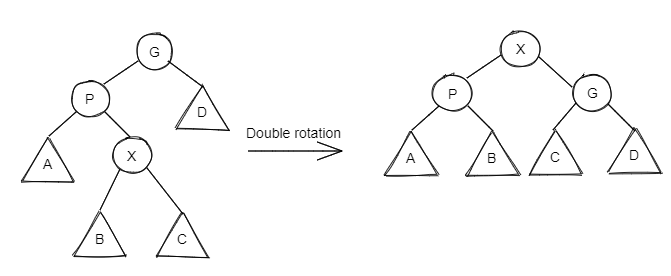
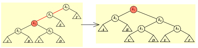
Case 2: P is not the root
- Zig-zag:
- Zig-zig:
第一个为 LR, 第二个为两次 LL
- Zig-zag:
-
那么对于开始的图形,使用 Splay 得到
Splaying not only moves the accessed node to the root, but also roughly halves the depth of most nodes on the path.
举个栗子
Deletions👀
- Step 1: Find X (X will be at the root)
- Step 2: Remove X (There will be two subtrees \(T_L\) and \(T_R\) )
- Step 3: FindMax( \(T_L\) ) (The largest element will be the root of \(T_L\) , and has no right child)
- Step 4: Make \(T_R\) the right child of the root of \(T_L\)
Amortized Analysis | 摊还分析👀
Abstract
Almost the most difficult question in ADS
- worst-case bound \(\ge\) amortized bound \(\ge\) average-case bound
- 分析方法:
- Aggregate analysis | 聚合分析
- Accounting method | 核算法
- Potential method | 势能方法 (Highest-level)
Aggregate Analysis👀
Show that for all n, a sequence of n operations takes worst-case time \(T(n)\) in total. In the worst case, the average cost, or amortized cost per operation is \(\frac{T(n)}{n}\)
Stack with MultiPop(int k, Stack S)
- Consider a sequence of \(n\) Push, Pop, and MultiPop operations on an initially empty stack. (sizeof(S) \(\le n\) )
- \(n\) 次操作, push 的操作 \(\le n\) (pop 必须要有 push), 最多的费用 \(\approx 2n-2\)
- \(T_{amortized} ~ = ~ O(n) / n ~ = ~ O(1)\)
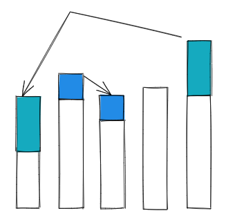
Accounting Method👀
- When an operation’s amortized cost \(\hat{c_i}\) exceeds its actual cost \(c_i\) , we assign the difference to specific objects in the data structure as credit (namely \(\Delta _i\)). Credit can help pay for later operations whose amortized cost is less than their actual cost.
- “劫富济贫”,将时间划分
柱状图表示各情况的时间费用
- \(\frac{\sum \hat{c_i}}{n} ~ = \frac{\sum c_i}{n} + \frac{\sum \Delta _i}{n} ~ \le ~ A\)
- 若希望 \(\frac{\sum \hat{c_i}}{n} \le A\) (A 为某个数值), 虽然 \(\Delta _i\) 取值都有可能,但如果 \(\frac{\sum \Delta _i}{n} \ge 0\) .
- 此时如果可以证明 \(\frac{max \sum \hat{c_i}}{n} \le A ~ \approx ~ \frac{\sum c_i}{n} \le A\) (其实就等价于计算最大的摊还费用 \(\le A\) , 即 worst-case 下费用 \(\le A\) )
Stack with MultiPop(int k, Stack S)
- \(c_i\) for Push: 1; Pop: 1; MultiPop: min(sizeof(S), k)
- \(\hat{c_i}\) for Push: 2; Pop: 0; MultiPop: 0
Starting from an empty stack —— Credits for
- Push: +1; Pop: -1; MultiPop: -1 for each +1 ( \(\sum Credits \ge 0\) )
- sizeof(S) \(\ge 0 ~~ \Rightarrow ~~ Credits \ge 0\)
- \(\Rightarrow ~~ O(n) = \sum\limits_{i=1}^n \hat{c_i} \ge \sum\limits_{i=1}^n c_i\)
- \(\Rightarrow ~~ T_{amortized} = O(n)/n = O(1)\)
Potential Method👀
- Take a closer look at the credit —— \(\hat{c_i} - c_i = Credit = \Phi(D_i) - \Phi(D_{i-1})\) ( \(\Phi \rightarrow Potential ~ function\) )
- \(\sum\limits_{i=1}^n \hat{c_i} = \sum\limits_{i=1}^n (c_i + \Phi (D_i) - \Phi (D_{i-1})) = (\sum\limits_{i=1}^n c_i) + \Phi (D_n) - \Phi (D_0)\)
- 其中, \(\Phi (D_n) - \Phi (D_0) \ge 0\) (我们希望做到 \(\Phi (D_0) = 0 ~,~ \Phi(D_n) \ge 0\) , \(\Phi(D_0)\) 是常数也没有问题)
- In general, a good potential function should always assume its minimum at the start of the sequence
Stack with MultiPop(int k, Stack S)
- \(D_i\) = the stack that results after the i -th operation
- \(\Phi (D_i)\) = the number of objects in the stack \(D_i\)
- 则 \(\Phi (D_i) \ge 0 = \Phi (D_0)\)
- Push: \(\Phi (D_i) - \Phi (D_{i-1}) = (sizeof(S) + 1) - sizeof(S) = 1\)
- \(\hat{c_i} = c_i + \Phi (D_i) - \Phi (D_{i-1}) = 1 + 1 = 2\)
- Pop: \(\Phi (D_i) - \Phi (D_{i-1}) = (sizeof(S) - 1) - sizeof(S) = -1\)
- \(\hat{c_i} = c_i + \Phi (D_i) - \Phi (D_{i-1}) = 1 - 1 = 0\)
- MultiPop: \(\Phi (D_i) - \Phi (D_{i-1}) = (sizeof(S) - k' ) - sizeof(S) = -k'\)
- \(\hat{c_i} = c_i + \Phi (D_i) - \Phi (D_{i-1}) = k' - k' = 0\)
- \(\sum\limits_{i=1}^n \hat{c_i} = \sum\limits_{i=1}^n O(1) = O(n) \ge (\sum\limits_{i=1}^n c_i) ~~ \Rightarrow ~~ T_{amortized} = O(n)/n = O(1)\)
[example] : Splay Trees: \(T_{amortized} = O(log N)\)
- \(D_i\) = the root of the resulting tree
- \(\Phi(D_i)\) : must increase by at most \(O(log N)\) over \(n\) steps, AND will also cancel out the number of rotations (zig: 1; zig-zag: 2; zig-zig: 2)
- \(\Phi(T) = \sum\limits_{i \in T} log~S(i)\) where \(S(i)\) is the number of descendants of \(i\) ( \(i\) itself included)
\(T\) 即 \(D(i)\) , \(log~S(i)\) called Rank of the subtree \(\approx\) Height of the tree
-
\(\Phi(T) = \sum\limits_{i \in T} Rank(i)\)
- Zig:
- \(\hat{c_i} = 1 + R_2(X) - R_1(X) + R_2(P) - R_1(P)\)
- \(\le 1 + R_2(X) - R_1(X)\) ( \(R_2(X)\) 表示旋转后的这个点的势函数)
-
Zig-zag:
- \(\hat{c_i} = 2 + R_2(X) - R_1(X) + R_2(P) - R_1(P) + R_2(G) - R_1(G)\)
- \(\le 2(R_2(X) - R_1(X))\)
\((a+b)^2 \ge 4ab ~~ \Rightarrow ~~ 2log~(a+b) \ge 2 + log~a + log~b\)
-
Zig-zig:
- \(\hat{c_i} = 2 + R_2(X) - R_1(X) + R_2(P) - R_1(P) + R_2(G) - R_1(G)\)
- \(\le 3(R_2(X) - R_1(X))\)
- [Theorem] : The amortized time to splay a tree with root \(T\) at node \(X\) is at most \(3(R(T) - R(X)) + 1 = O(log~N)\)
- Zig: